Example Output
dRep produces a variety of output in the work directory depending on which operations are run.
To generate the figures below, dRep dereplicate was run on a set of 5 randomly chosen Klebsiella oxytoca isolate genomes as follows:
$ dRep dereplicate complete_only -g *.fna --S_algorithm gANI
See also
- Overview
- for general information on the program
- Quick Start
- for more information on dereplicate_wf
- Module Descriptions
- for a more detailed description of what the modules do
Figures
Figures are located within the work directory, in the folder figures:
$ ls complete_only/figures/
Clustering_scatterplots.pdf
Cluster_scoring.pdf
Primary_clustering_dendrogram.pdf
Secondary_clustering_dendrograms.pdf
Winning_genomes.pdf
Primary_clustering_dendrogram
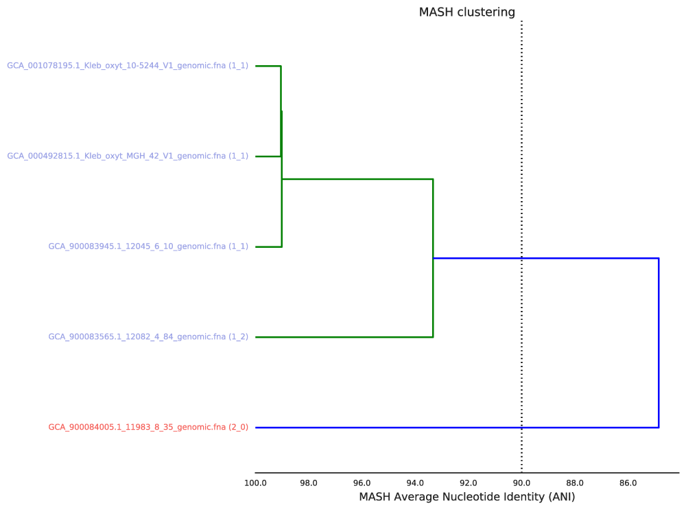
The primary clustering dendrogram summarizes the pair-wise Mash distance between all genomes in the genome list.
The dotted line provides a visualization of the primary ANI - the value which determines the creation of primary clusters. It is drawn in the above figure at 90% ANI (the default value). Based on the above figure you can see that two primary clusters were formed- one with genomes colored blue, and one red.
Note
Genomes in the same primary cluster will be compared to each other using a more sensitive algorithm (gANI or ANIm) in order to form secondary clusters. Genomes which are not in the same primary cluster will never be compared again.
Secondary_clustering_dendrograms
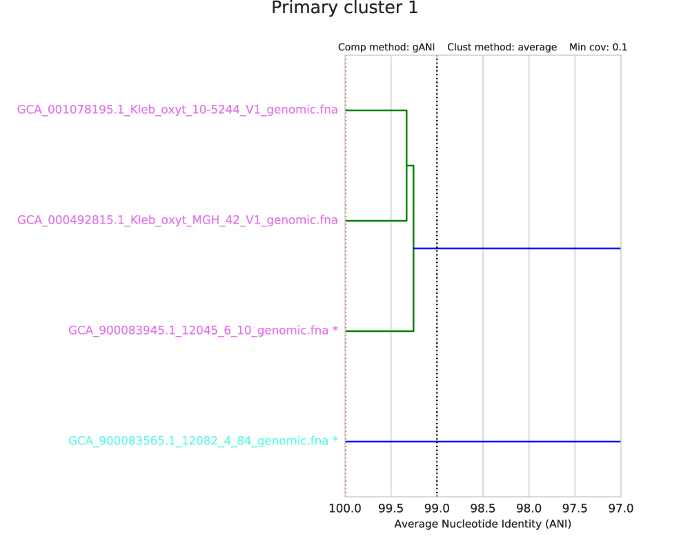
Each primary cluster with more than one member will have a page in the Secondary clustering dendrograms file. In this example, there is only one primary cluster with > 1 member.
This dendrogram summarizes the pair-wise distance between all organisms in each primary cluster, as determined by the secondary algorithm (gANI / ANIm). At the very top the primary cluster identity is shown, and information on the secondary clustering algorithm parameters are shown above the dendrogram itself. You can see in the above figure that this secondary clustering was performed with gANI, the minimum alignment coverage is 10%, and the hierarchical clustering method is average.
The black dotted line shows the secondary clustering ANI (in this case 99%). This value determines which genomes end up in the same secondary cluster, and thus are considered to be the “same”. In the above figure, two secondary cluster are formed. The “best” genome of each secondary cluster is marked with as asterisk.
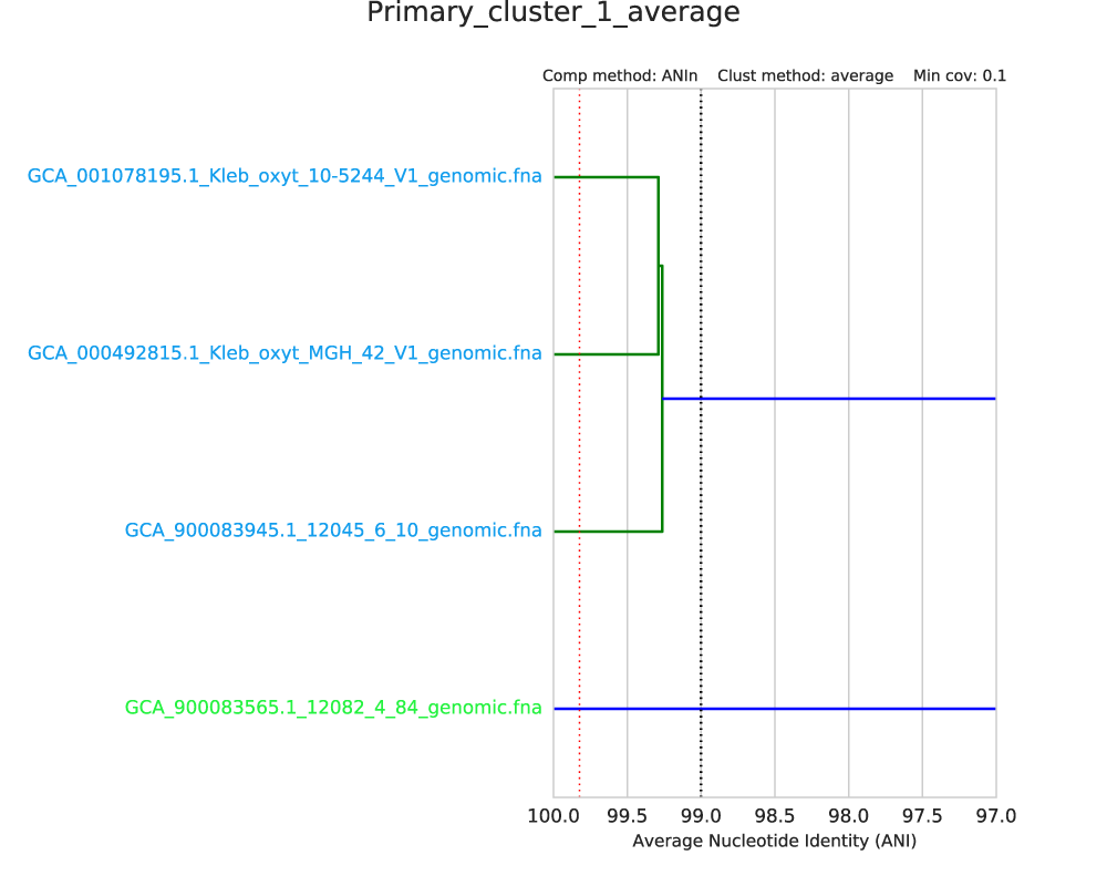
The red line shows the lowest ANI for a “self-vs-self” comparison of all genomes in the genome list. That is, when each genome in this primary cluster is compared to itself, the red line is the lowest ANI you get. This represents a “limit of detection” of sorts. gANI always results in 100% ANI when self-vs-self comparisons are performed, but ANIm does not (as shown in the figure below).
Cluster_scoring
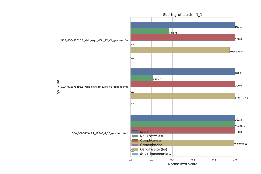
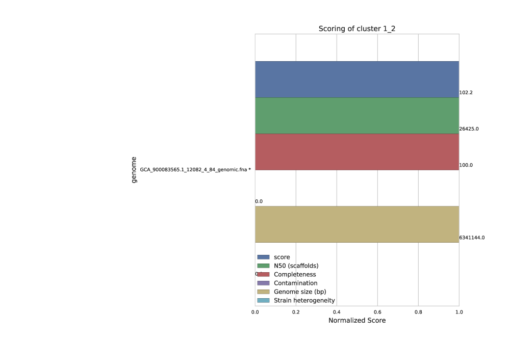

Each secondary cluster will have its own page in the Cluster scoring figure. There are three secondary clusters in this example- 2 of which came from primary cluster 1, and 1 of which is the only member of primary cluster 2.
These figures show the score of each genome, as well as all metrics that can go into determining the score. This helps the user visualize the quality of all genomes, and ensure that they agree with the genome chosen as “best”. The “best” genome is marked with an asterisk, and will always be the genome with the highest score.
One genome will be selected from each secondary cluster to be included in the de-replicated genome set. So in the above example, we will have 3 genomes in the de-replicated genome set. This is because the algorithm decided that all genomes in cluster 1_1 were the “same”, and chose GCA_900083945 as the “best”.
See also
See Module Descriptions for information on how scoring is done and how to change it
Other figures
Clustering scatterplots provides some information about genome alignment statistics, and Winning genomes provides some information about only the “best” genomes of each replicate set, as well as a couple quick overall statistics.
Warnings
Warnings look for two things: de-replicated genome similarity and secondary clusters that were almost different. All warnings are located in the log directory within the work directory, in a file titled warnings.txt
de-replicated genome similarity warns when de-replicated genomes are similar to each other. This is to try and catch cases where similar genomes were split into different primary clusters, and thus failed to be de-replicated.
secondary clusters that were almost different alerts the user to cases where genomes are on the edge between being considered “same” or “different”. That is, if a genome is close to one of the differentiating lines in the Primary and Secondary Clustering Dendrograms shown above.
Other data
The folder dereplicated_genomes holds a copy of the “best” genome of each secondary cluster
See also
Almost all data that dRep generates at any point is able to be accessed by the user. This includes the full checkM results of each genome, the value of all genome comparisons, the raw hierarchical clustering files, the primary and secondary cluster identity of each genome, etc.
For information on where all of this is stored, see Advanced Use